Pathway to continual learning: Delta Attention state as Fast Programmable Weights

Moonshot with its KDA is onto bigger things, and most are missing it..

Inspiration

This post is dedicated to Dwarkesh Patel. He continuously keep bringing up the topic of continual learning with his guests. As he rightly points out, we can not say we have arrived at AGI unless we solve continual learning. There have been many mechanism for continual learning. Some involve building external memories, but until models can not learn to update their weights with every single interaction - just the way human re-wire neural pathway with every interaction - we can not really say we have arrived at AGI.

Preface

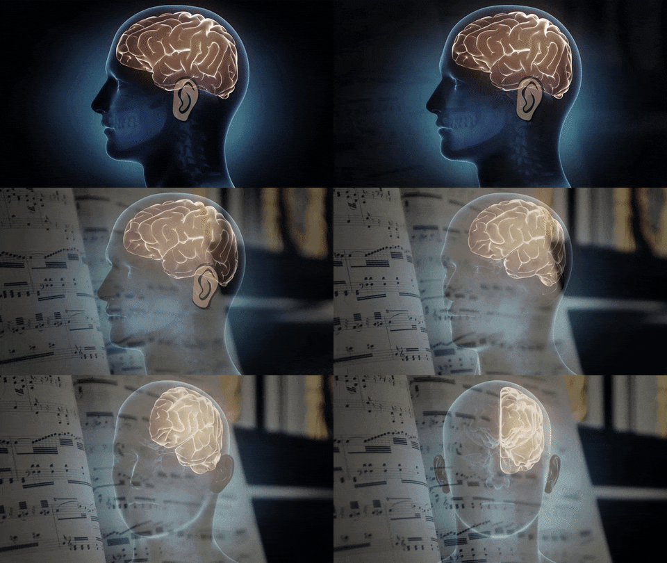
Continual learning is, in my view too, the holy grail for AGI. A model that cannot learn after deployment is frozen at its training cutoff - every hour it is used produces no durable improvement, and every new interaction starts from the same blank slate. An LLM model that accumulates the model of its world from its own experience, without a retraining run would be a massive leap over today’s models and help us arrive at AGI.

The observation that started this essay are simple facts about Kimi' K3: No ROPE and fixed state.
1. First of all, no ROPE means practically infinite context (in theory).
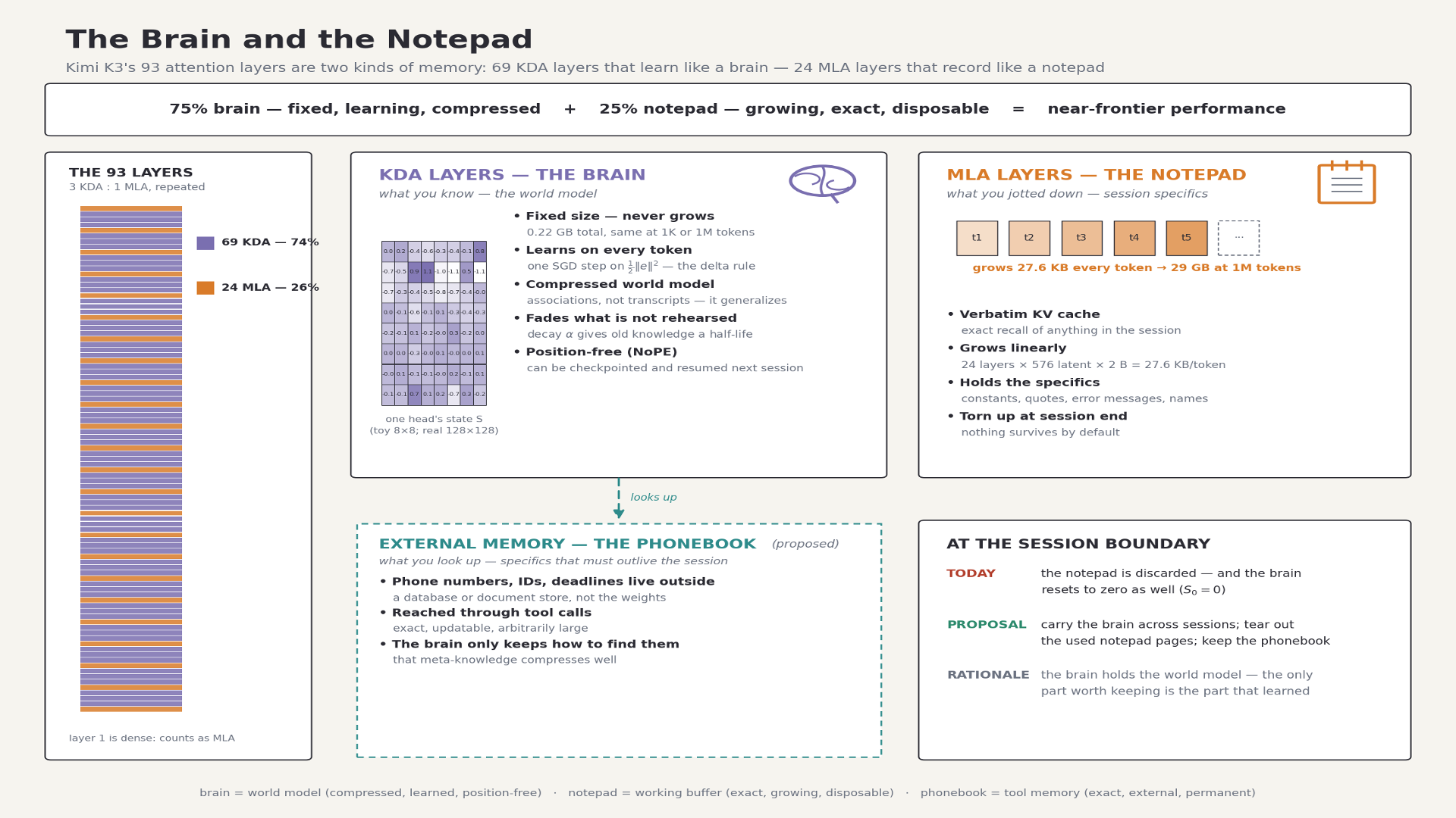
2. Of K3’s 93 attention layers, 69 i.e. about 75% are KDA layers whose entire memory is a fixed: 128 × 128 state matrix per head, however long the context gets. Only 24 layers i.e. 25% are Gated MLA layers with a KV cache that grows linearly with context. What is so special about K3 is despite having 75% KDA or linear layers, it performs near the frontier - it is the first model to do that. In other words, three quarters of the model’s attention runs on fixed-size, lossy, compressed memory (KDA) without giving up much capability; exact token-level cache in every layer is apparently not required for the frontier performance!

There is a familiar analogy. The human brain is also a fixed-size container, and we plainly do not remember everything that happens to us: we keep the important ideas, let the rest go, and what we retain is less a recording than an updated world model. For the details we cannot afford to keep, we rely on external media — phonebooks are a classic example. Our intelligence lives mostly in a compressed model, not in an archive. KDA works the same way: bounded capacity, error-driven updates, decay that keeps what is rehearsed and fades what is not, generalisation instead of verbatim storage.

Fixed storage in brain for ideas and external storage for data

Having known Yang Zhilin’s work (CEO Moonshot), he is not making choices these choices (like KDA, no ROPE) lightly!!! He could have simply followed DeepSeek’s MLA + DSA and scaled the model, but he did not…

While Kimi K3’s KDA shows a pathway towards continual learning with its fixed state that we will explore in detail, none of the core idea is specific to KDA only: any delta-rule linear attention has the same structure and same potential.. The idea of Linear transformers (Kimi K3 is Hybrid Linear - we will see more details soon) acting as fast weight programmers was articulated by Imanol Schlag, Kazuki Irie, and Jürgen Schmidhuber in their paper: Linear Transformers Are Secretly Fast Weight Programmers (2021), building on Schmidhuber’s fast-weight idea from 1992. While the idea may seem old, it was not taken as a serious idea, as Linear Transformers themselves were not mainstream. What Kimi’s KDA did was to give a proof that you can achieve frontier performance, making the idea mainstream now. This essay takes that 2021 observation, and asks concretely what it would take to turn that idea into a full blown continual learning architecture to take us to AGI.

Trivia: did you recognise who is the third person mentioned on the above paper? Yep!

What follows is a deep dive essay about a significant aspect of Kimi K3 i.e. its KDA state. It is not just a cache-able state, but a set of fast weights, trained by gradient descent on every token the model processes. Making it persistent is a plausible path to continual learning.

We see topics in the below order: the mechanism (§3), the exact loss and gradient that make the update a learning rule (§4), why the absence of RoPE helps (§5), three design proposals toward ‘real’ continual learning (§7), and the capacity and systems limits I see (§8).

Contents

Introduction

1. The problem: deployed models do not learn

2. Kimi K3 in brief

3. The KDA state, mechanically

4. The update is gradient descent on a loss

5. Why the absence of RoPE matters here

6. The thesis: the state is a world model in fast weights

7. Three proposals toward continual learning

8. Should we have a bigger state? How big a state we could have?

9. Summary

1. The problem: deployed models do not learn

A deployed language model has exactly two places where information about the current interaction can live. The first is the weights, which are frozen after training: they encode everything the model learned from its training corpus, and they do not change when you talk to the model. The second is the context — the token history in the prompt, together with the per-layer KV cache built from it. The context is writable: every new token adds to it, and the model can attend back to anything in it. But it is temporary. When the session ends, the cache is discarded, and the next session starts from the frozen weights plus nothing.

Continual learning means closing the gap between these two stores: the model should keep something it learned during deployment, across session boundaries, without a retraining run. Fine-tuning on user data is one answer, but it is offline, expensive, and risks catastrophic forgetting of the base weights. The interesting question is whether the architecture itself already contains a writable, persistent memory that is more compact and more “weight-like” than a raw token history.

Kimi K3’s attention design contains exactly such an object: the KDA state. It is a fixed-size matrix per attention head that is updated on every token by an explicit learning rule — one that is mathematically identical to an SGD step on a per-token loss.

2. Kimi K3 in brief (you may skip)

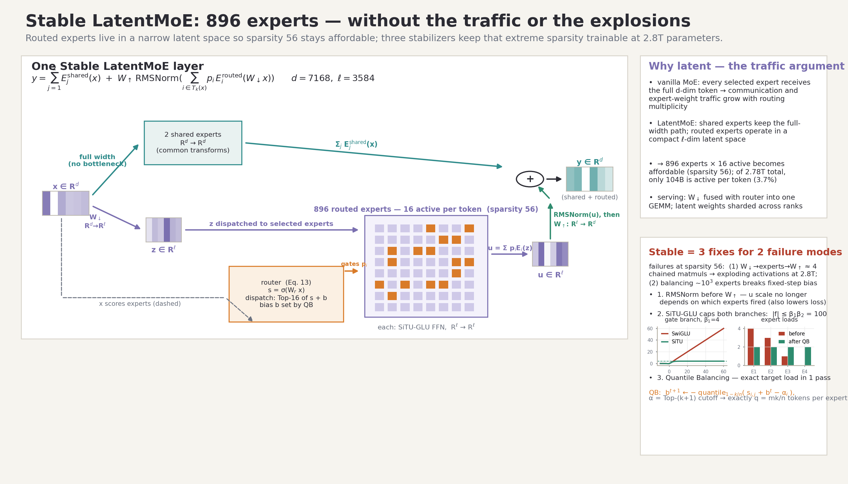
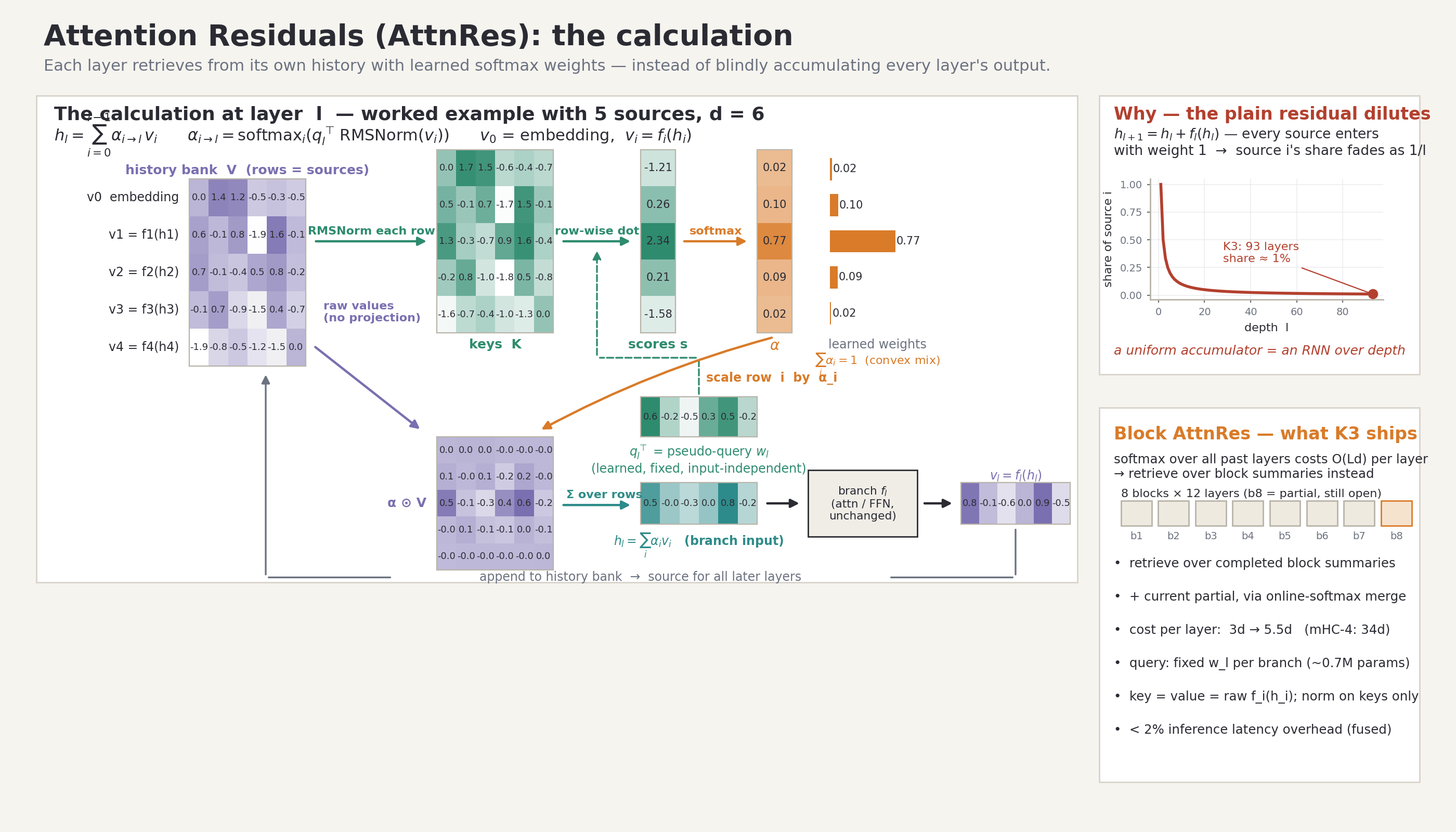
Kimi K3 is a 2.8-trillion-parameter mixture-of-experts model with 104B active parameters per token, 93 layers, and a 1M-token context window. Its attention is hybrid: 69 KDA (Kimi Delta Attention) layers interleaved with 24 Gated MLA layers in a 3:1 pattern — the ratio that Kimi Linear’s ablations found optimal. The MoE backbone (Stable LatentMoE, 896 routed experts with 16 active per token) and the cross-depth Attention Residuals are important to K3 but mostly orthogonal to this article’s argument; the two diagrams below are included for orientation.

K3’s feed-forward side. Routed experts operate in a narrow latent space so that 896-expert sparsity stays affordable at 2.8T parameters. This is where most of the frozen knowledge lives; it is not the subject of this article, but it sets the scale contrast for §8: the writable KDA state is about four orders of magnitude smaller than the frozen weights.

Attention Residuals. Each layer retrieves from a bank of earlier layers’ outputs with learned softmax weights, instead of the plain residual stream accumulating every layer with weight 1. AttnRes moves information across depth; KDA moves information across time. Continual learning is about the time axis, so KDA is the focus from here on.

The two attention types maintain very different runtime memories. Each Gated MLA layer keeps a standard KV cache (in latent form) that grows by a fixed amount per token. Each KDA layer keeps a fixed-size state matrix per head — d_k × d_v = 128 × 128 — no matter how long the sequence gets. The total memory picture per request:

Per-request memory. An all-MLA model of the same depth would need 107 KB of cache per token; K3 needs 27.6 KB/token for its 24 MLA layers plus a fixed 0.22 GB of KDA state (69 layers × 96 heads × 128 × 128 × 2 bytes ≈ 217 MB), independent of context length. Two facts in this figure drive everything below: the KDA state is fixed-size, and it is small.

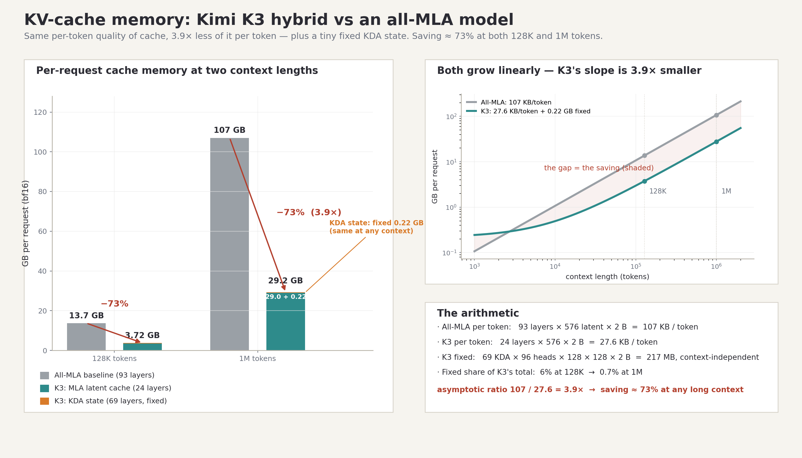
So K3 already splits its runtime memory into a growing part (MLA cache) and a constant part (KDA state). The proposal developed later is, in essence, to make that split semantic as well: session-specific detail in the growing part, long-term learned structure in the constant part — and to carry the constant part across sessions.

3. Understanding the KDA state update

Each KDA head maintains a state matrix S_t ∈ ℝ^d_k×d_v. For each incoming token the head produces four vectors from its projections: a key k_t, a value v_t, a per-channel decay α_t ∈ (0,1)^d_k, and a write strength β_t. The state then advances by

S_t= (I− β_tk_tk_t^⊤) Diag(α_t)S_t−1+ β_tk_tv_t^⊤(1)

Reading (1) right to left, three things happen per token:

One token, one head. ① Forget: Diag(α_t) scales every row (channel) of the old state by its own decay — a per-channel clock, finer-grained than the scalar gates of earlier delta nets. ② Erase: the rank-1 downdate (I − β_tk_tk_t^⊤) removes only the component of memory that lies along the new key direction — other keys’ associations are untouched. ③ Write: a rank-1 outer product stores the new association k_t ↦ v_t. The bottom panels show the readout and the two useful views of the same matrix: rows are the memory channels, columns are what the erase touches.

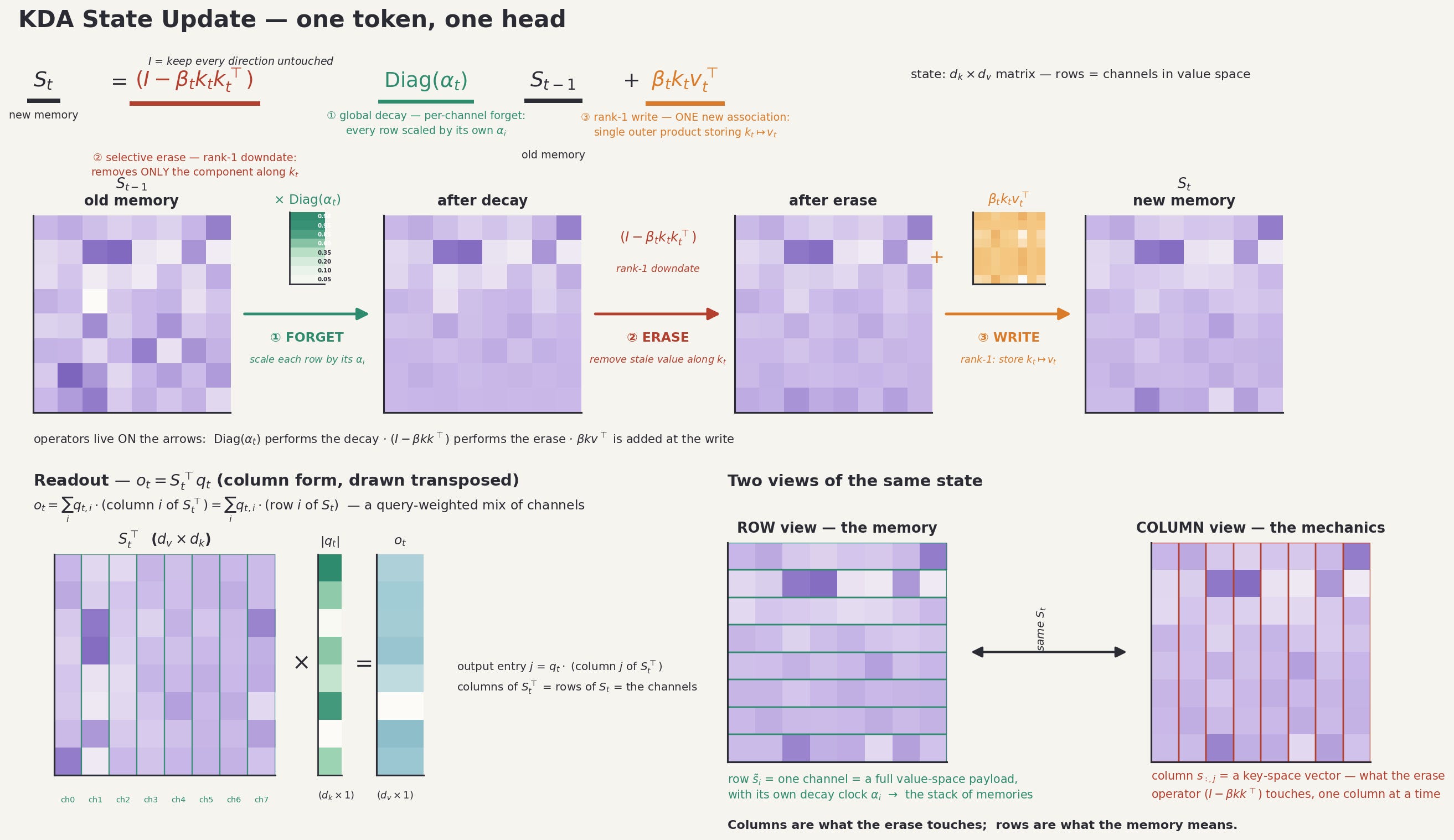
Reading from the state is a matrix–vector product. A query vector q_t produces the output o_t = S_t^⊤q_t: a query-weighted mixture of the state’s rows. The same operation written as a row vector, o_t^⊤ = q_t^⊤S_t, is how the chunkwise kernel computes it for many tokens at once:

Two ways to write the same readout. Column form (probe view): each output entry is a dot product of q_t with one column of S_t. Row form (stack-of-memories view): each coordinate of q_t scales one row, and the rows are summed. Identical numbers — verified to be exactly equal.

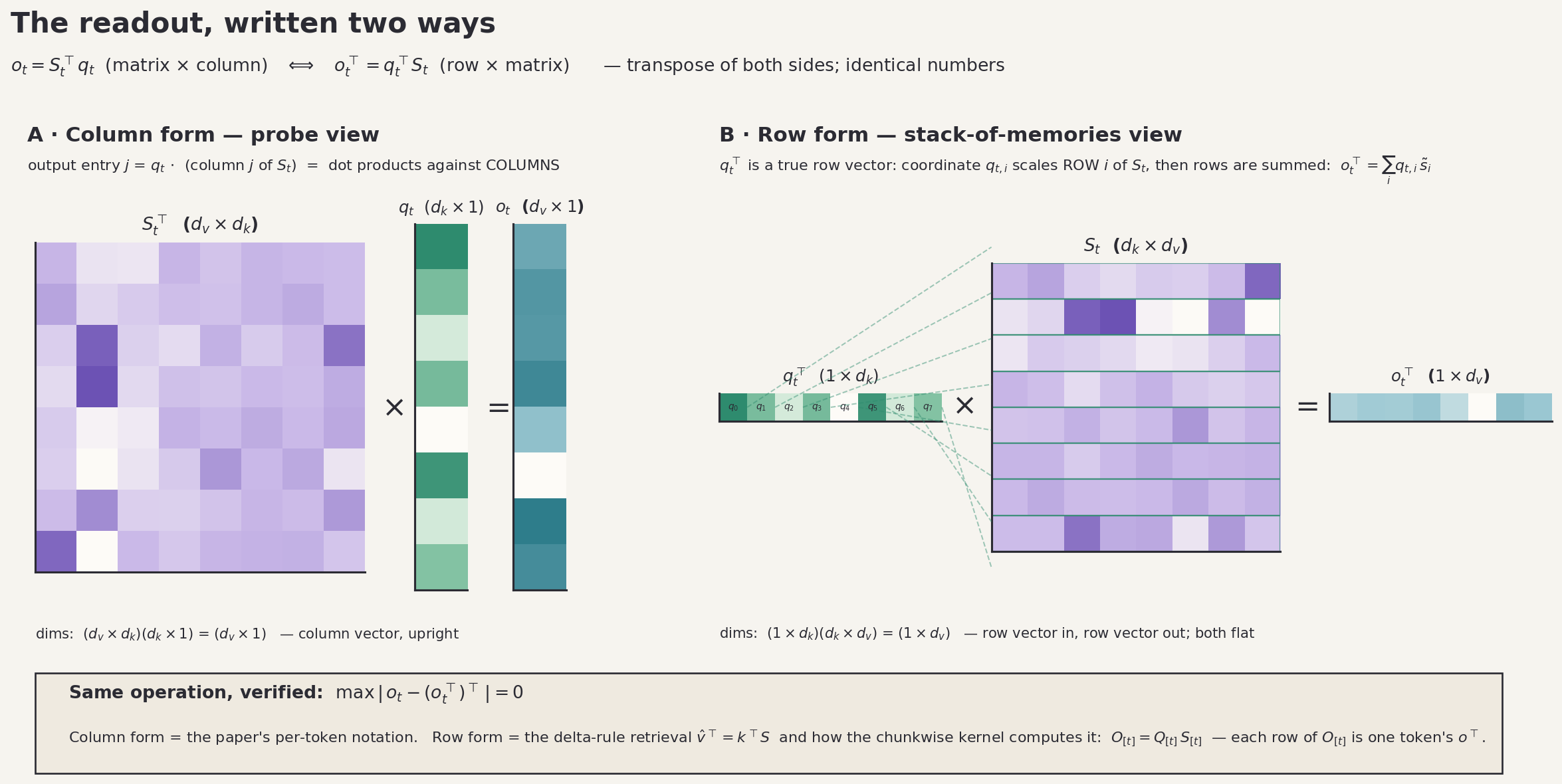
The readout is what the rest of the network consumes at inference time. The diagram below shows the full read path, and contrasts it with the write path:

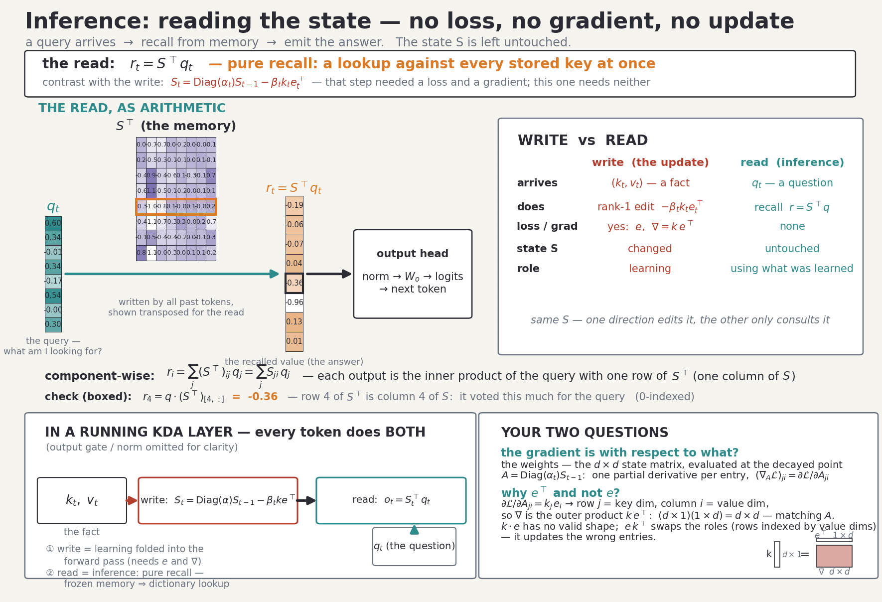
Two properties matter for everything that follows.

1. First, the state has fixed size: whether the model has seen a hundred tokens or a million, the memory is the same 128 × 128 matrix per head — all past experience is compressed into it, lossily.

2. Second, the update is local in time: S_t depends only on S_t−1 and the current token’s vectors. There is no replay buffer, no attention over history, no second pass. These are exactly the properties of an online learning system, and the next section shows that this is not an analogy but an identity.

4. Re-interpretation: The KDA state update is gradient descent on a loss

This section is very technical, you can directly jump to the last diagram in this section to see the results.

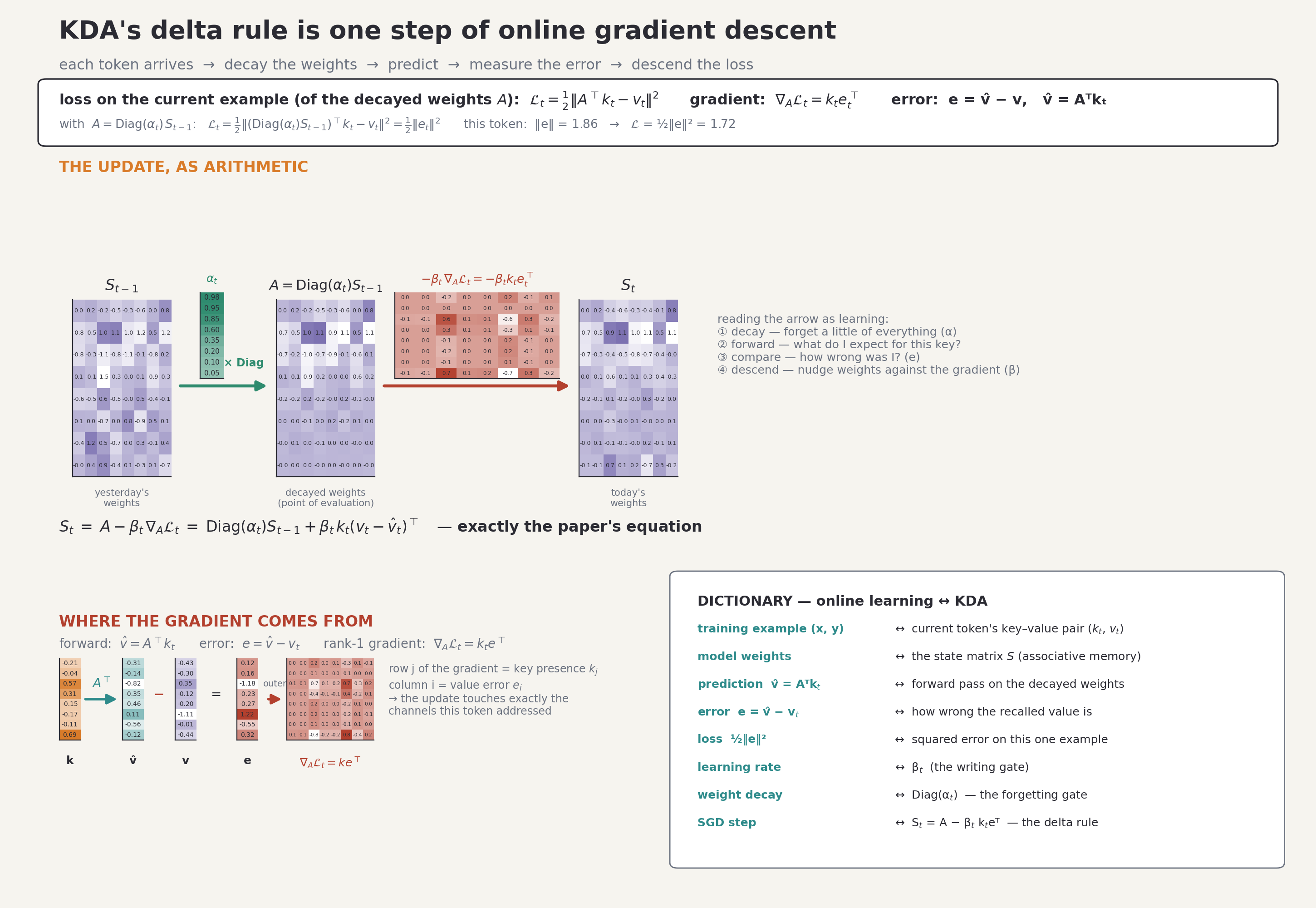
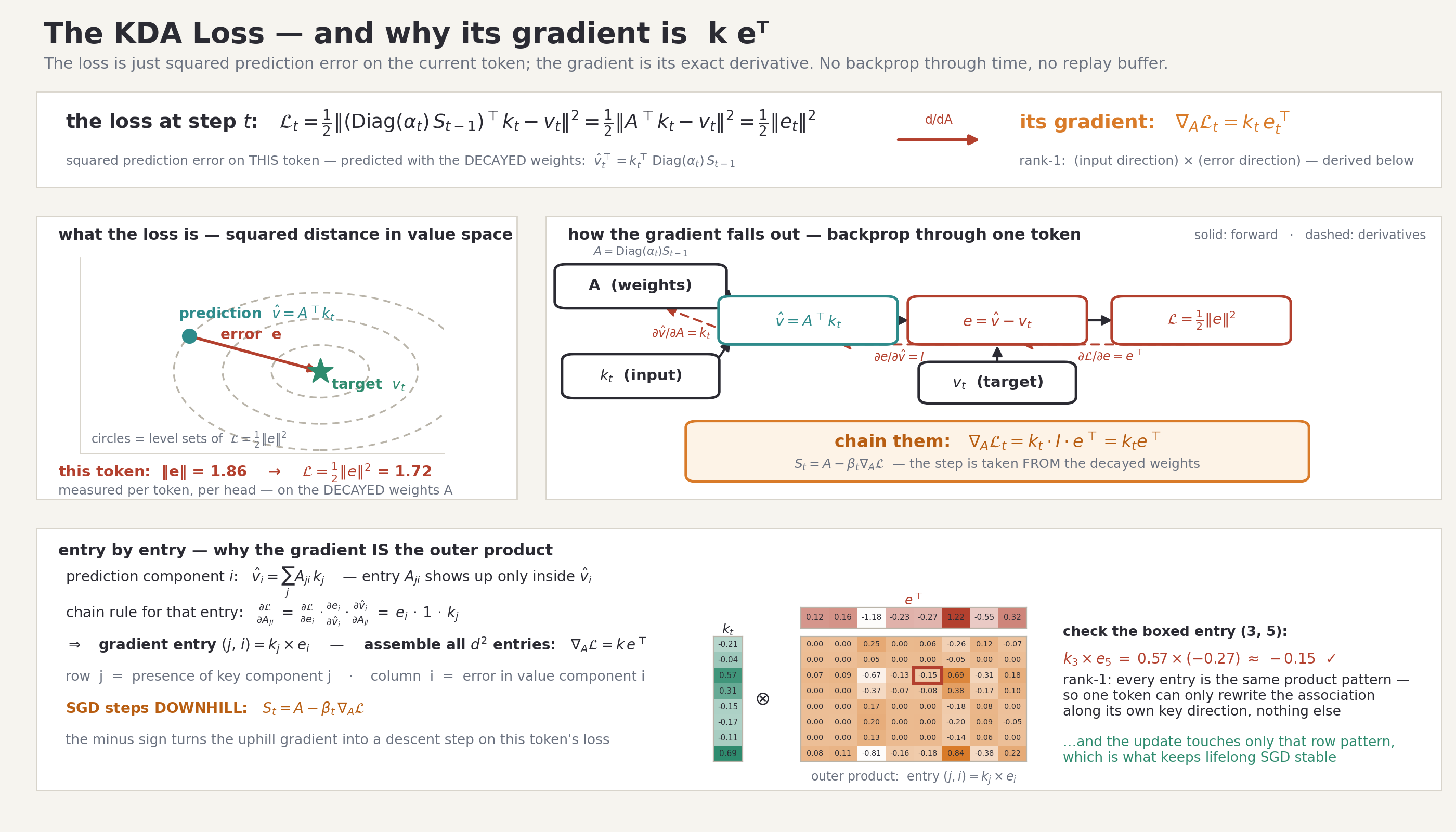
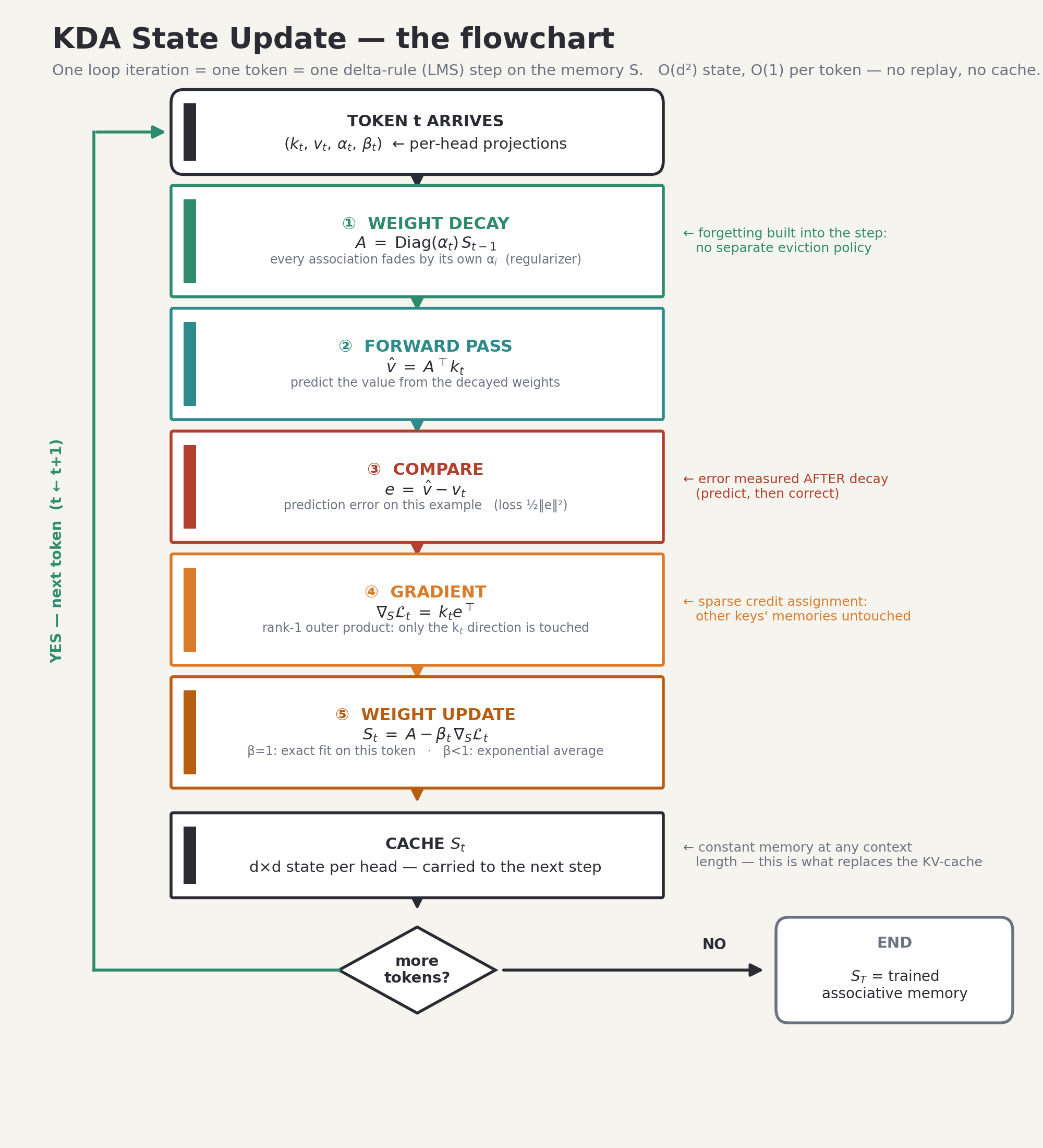
Define the decayed weights A = Diag(α_t)S_t−1 — the state after the forget step, before the new token is written. Before writing, the head predicts the current token’s value from its key using those weights: v̂ = A^⊤k_t. The prediction error is e_t = v̂ − v_t. Now score that prediction with a squared loss on the decayed weights:

L_t= ½‖A^⊤k_t−v_t‖² = ½‖e_t‖²(2)

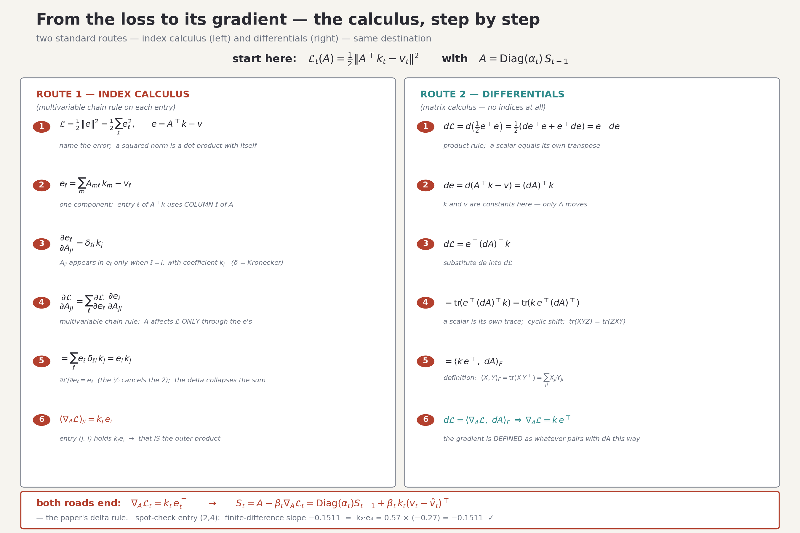
Differentiating (2) with respect to the matrix A gives a rank-1 gradient (derived entry by entry below):

∇_AL_t=k_te_t^⊤(3)

and one SGD step from the decayed weights, S_t = A − β_t∇_AL_t, is exactly the update (1): the erase term is the part of the gradient step that removes the stale prediction along k_t, and the write term is the part that installs the corrected value.

The KDA recurrence is online gradient descent — specifically the classical delta rule (Widrow–Hoff LMS, 1960) with a per-channel weight-decay regularizer — run on the model’s own activations, at inference time, on every token. The following diagrams unpack each piece of that claim.

The learning view. Top banner: the loss is taken on the decayed weights A = Diag(α_t)S_t−1, and its gradient is the outer product k_te_t^⊤ — note the operator placement, A^⊤ acts on the key to produce the prediction. Main panel: one token’s update computed numerically — decay, predict, compare, correct — with the four quantities shown as heatmaps.

Why the gradient is an outer product. Left: the loss is squared distance in value space between prediction and target. Right: backprop through one token — ∂L/∂e = e^⊤, ∂e/∂v̂ = I, ∂v̂/∂A involves k_t — chains to k_te_t^⊤. Bottom, entry by entry: gradient entry (j, i) = k_j × e_i, checked numerically. The practical consequence: one token can only rewrite the association along its own key direction — sparse credit assignment, which is what keeps lifelong SGD stable.

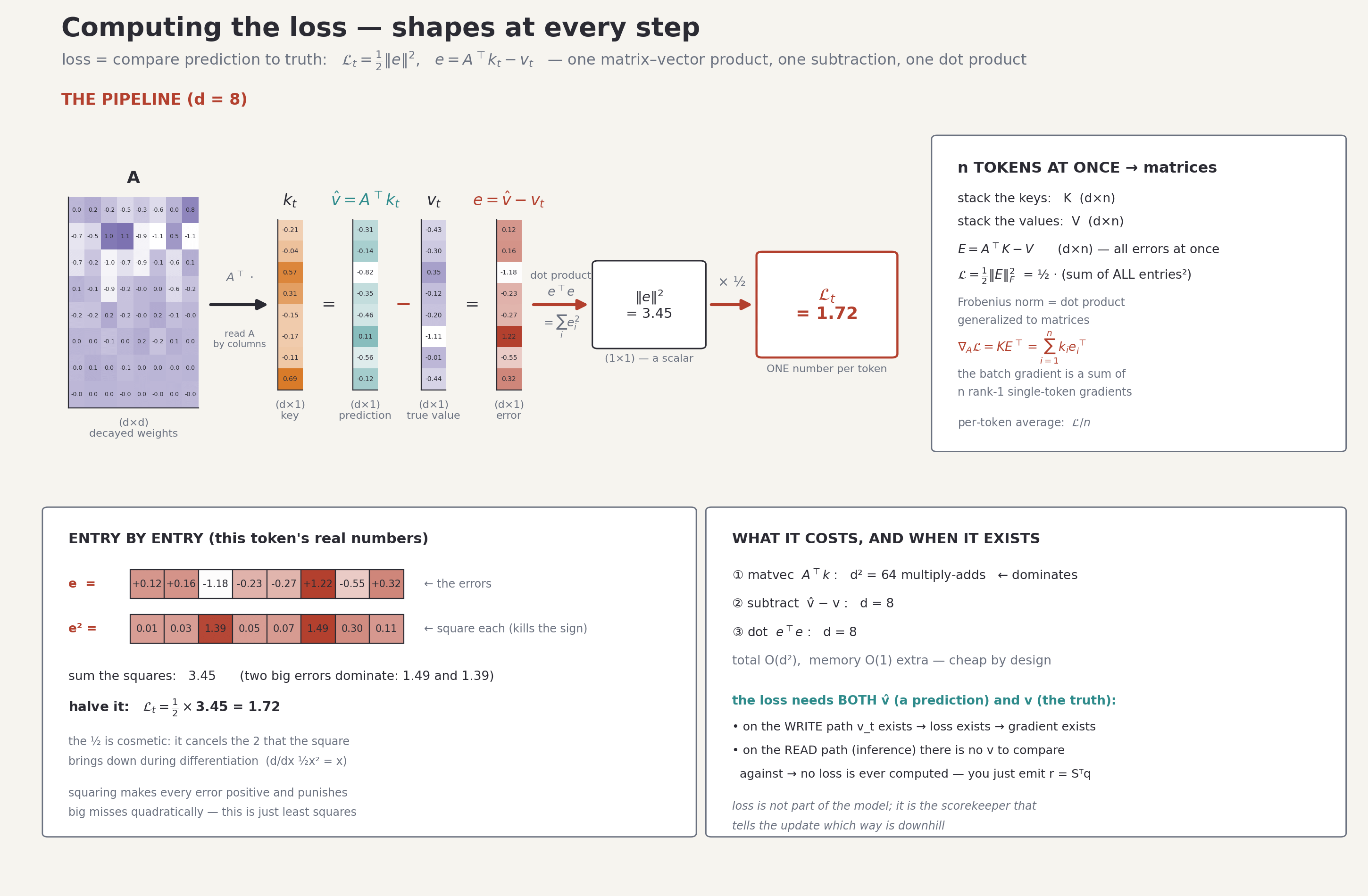
The loss involves matrices and vectors but is itself a scalar — it is just a sum of squared entry-wise errors, and the batch version replaces the vector error with an error matrix and the norm with the Frobenius norm:

The loss, shape by shape. Top: the single-token pipeline from A through k, v̂, v to the scalar L. Middle: the batch form — K, V, E = A^⊤K − V, L = ½‖E‖²_F, and ∇_AL = KE^⊤ = Σ_i k_ie_i^⊤, a sum of rank-1 terms. Bottom: entry-by-entry computation and the O(d²) cost.

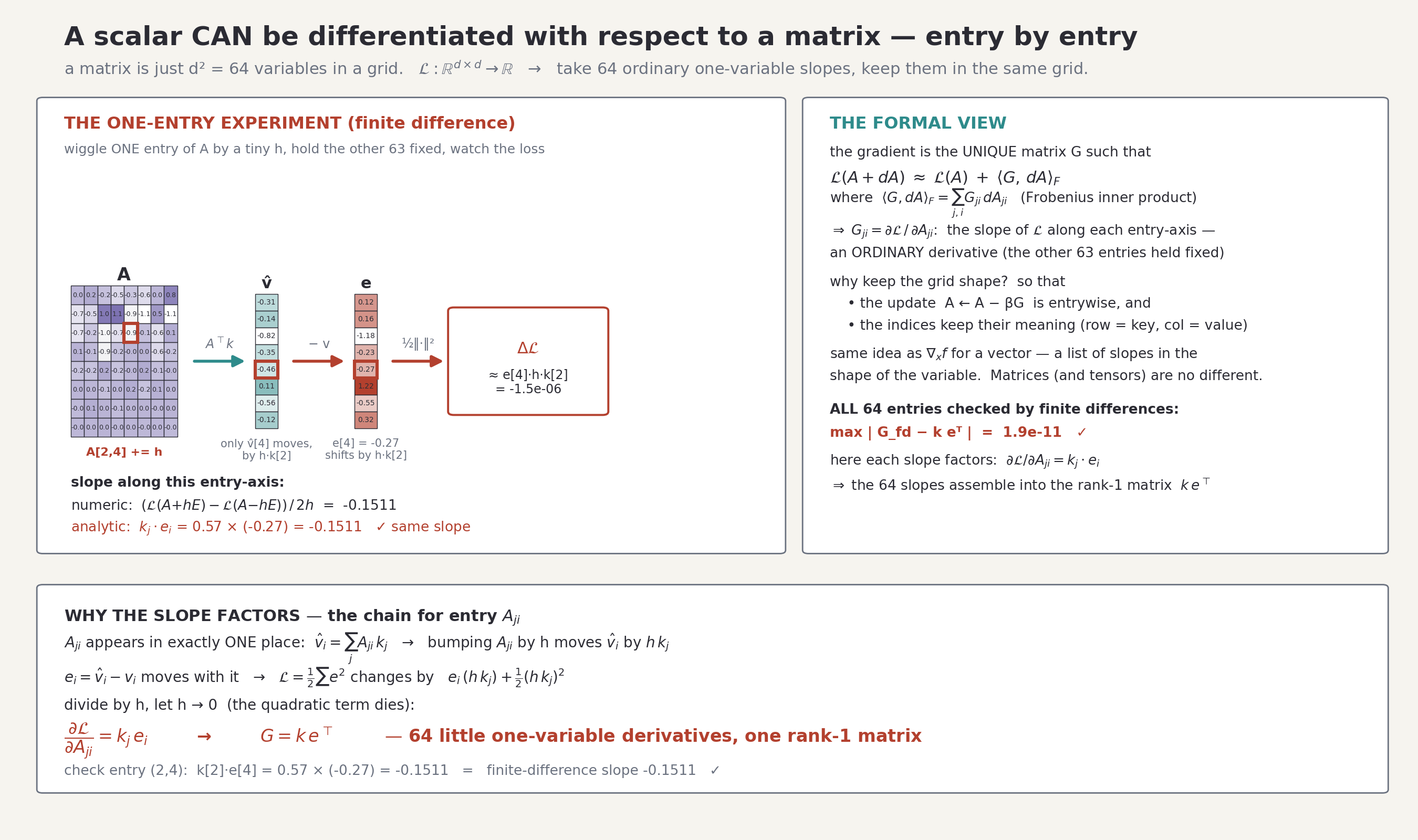
Differentiating a scalar with respect to a matrix is defined entry-wise: the gradient is the matrix of partial derivatives, equivalently the unique matrix G satisfying dL = ⟨G, dA⟩_F under the Frobenius inner product. Both views, and a finite-difference check on all 64 entries of a toy state:

Scalar loss, matrix argument. Left: perturbing one entry A_2,4 and measuring the loss change reproduces the analytic gradient entry k₂e₄ to eleven decimal places. Right: the formal view — the gradient is defined by the Frobenius pairing dL = ⟨G, dA⟩_F; all 64 entries verified, max error 1.9e-11.

For completeness, the full derivation from the loss equation to k_te_t^⊤, by two independent routes - index calculus with the Kronecker delta, and matrix differentials with the trace trick:

Two derivations. Route 1 (index calculus): write L in components, differentiate e_ℓ with respect to A_ji (the Kronecker delta δ_ℓi selects which error component each weight entry feeds), apply the chain rule, watch the sums collapse to k_je_i. Route 2 (differentials): dL = e^⊤de, substitute de = (dA)^⊤k, cycle the trace, read off G from the Frobenius pairing. Both land on the paper’s update equation.

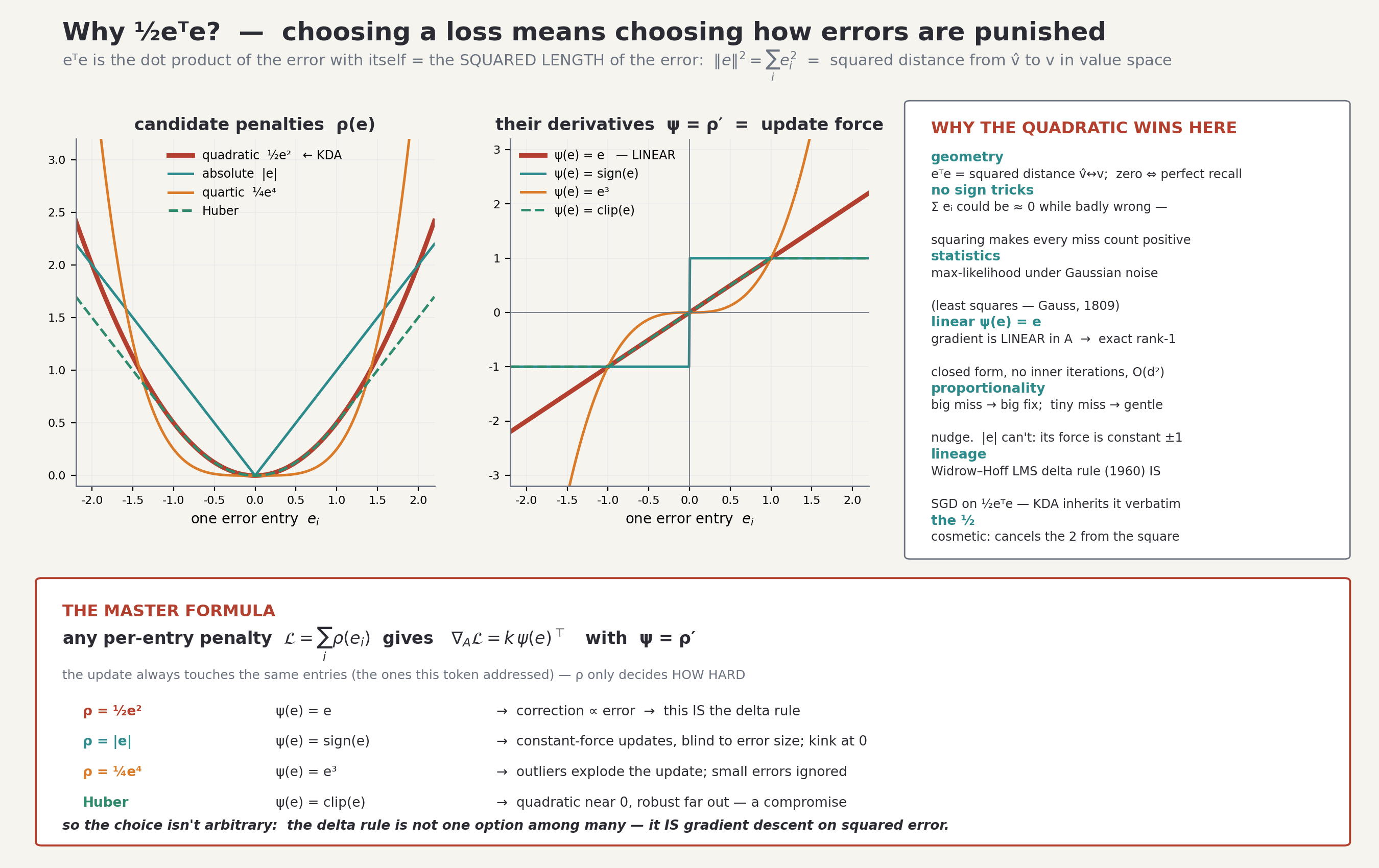
Finally: why this loss and not another? Because any per-entry penalty ρ(e) produces a gradient of the same rank-1 form, k ψ(e)^⊤ with ψ = ρ′ — and the quadratic is the unique choice whose derivative is the identity, making the update linear in the error, exactly the delta rule:

Why ½e^⊤e. Left: candidate penalties (quadratic, L1, quartic, Huber) and their derivatives. Right: the master formula ∇_AL = k ψ(e)^⊤ — only ψ(e) = e gives a linear update; the quadratic is also the Gaussian maximum-likelihood choice and the one whose single step with β = 1 fits the current example exactly. The squared loss is what makes KDA a clean online least-squares learner.

The whole loop on one page. One iteration = one token = one LMS step on the memory: decay (regularizer), forward pass (predict), compare (error), gradient (rank-1), weight update, cache the state, advance. O(d²) state, O(1) work per token, no replay, no growing cache. The endpoint S_T is a trained associative memory — the object this article is about.

5. Why the absence of RoPE matters here?

K3’s attention layers use no rotary position embedding. In the Kimi Linear design this is deliberate: the MLA layers are NoPE, and positional/recency information is carried entirely by the KDA layers’ data-dependent decay gates — ablations found NoPE with KDA outperforming RoPE, and RoPE base-frequency sensitivity is a known complication for context extension. This has a specific consequence for continual learning.

A RoPE-based memory encodes position into every cached key: a fact learned at position 50,000 of session 1 is stored rotated by 50,000 steps. Resuming such a cache in session 2 either continues the position counter (positions drift ever upward, into regimes the model may extrapolate poorly to) or resets it (every cached key is now mis-rotated). The KDA state has no such coupling. Recency in (1) is expressed by how many decay steps an association has survived, not by where it occurred. An association written a million tokens ago and never refreshed has simply faded by the product of the α’s along the way — the same fading whether those tokens were in one session or ten. The state is therefore a position-free checkpoint: it can be saved at the end of one session and loaded at the start of another with no re-indexing, no counter bookkeeping, and no rotational inconsistency. Whatever the state’s other limitations (§8), position handling is not one of them — an accidental but real enabler for the proposals below.

6. The thesis: the state is a world model in fast weights

Sections 3–5 establish the mechanism. Now we make the claim.

The frozen weights of K3 are a world model in the usual sense: compressed statistics of the training corpus, distilled by gradient descent over months of compute. The KDA state is the same kind of object at a different scale and speed. It is a set of fast weights: matrices that are not trained offline but are trained by the forward pass itself, one SGD step per token, on a prediction loss defined over the model’s own activations. Over a session, the state matrices across all heads in 69 layers accumulate a compressed, associative model of that session’s world: the documents read, the entities discussed, the corrections the user issued, the structure of the task.

Three properties make this look like a continual-learning substrate rather than just a cache:

• It learns by gradient descent. The update is not bookkeeping (append, evict); it is error-driven. The state moves downhill on a loss, which is what “learning” means everywhere else in the model.

• It generalizes by construction. The state does not store tokens; it stores directions in representation space. A probe key similar — not identical — to a written key retrieves a similar value, because the memory is a linear operator, not a table. This is the difference between a world model and a transcript.

• It is bounded and position-free. Fixed size means the cost of carrying it never grows; NoPE means carrying it across sessions is well-defined (§5).

There is one obvious gap between this and continual learning: today the state is thrown away at the end of a session. While the state is maintained across several interactions within a session, at the first token/interaction of a new session, every KDA head starts from S₀ = 0 and relearns the world from scratch. The machinery for accumulation exists; the persistence does not. The next section is about closing that gap.

Kimi K3: KDA (75% layers) is the brain and MLA layers (25% layers) are the notepad. We also need external memory that is practically infinite in its size.

7. Three proposals toward continual learning

Proposal 1 — the state-handoff experiment

Retain the KDA state across sessions while discarding the MLA KV cache, and measure what survives. The current serving arrangements reset both: for new session, we start with zero state and no MLA KV cache. The experiment changes one bit: at a session boundary, checkpoint all 69 (layers) × 96 (heads) state matrices (~0.22 GB total today, proposed to increase at least 10 times in the following text), drop the MLA cache entirely, and initialise the next session from the checkpoint instead of zeros.

Construct session 1 to teach the model things it cannot know from pre-training — a synthetic project’s conventions, a new codebase’s layout, a user’s preferences, fictional entities with defined properties. Then in session 2 initiated with KDA state from the first session, but with no MLA KV cache (25% of layers) and no repeated context, probe: does the model behave as if it knows these things? It is likely to remember a few details from the KDA state. However, in deep learning we can always train the model what we want, provided we have a dataset for tasks and know how to compute loss. So, we will need to create tasks that use KDA state from past sessions, and prompts that do not repeat knowledge that is likely to be in that KDA state.

Another direction is to eliminate MLA completely, as it complicates such adaptations. The model could only have large KDA states (discussed more in section 8.2) across 100% of the layers, with a tool to retrieve specific details from the past context.

Proposal 2 — disentangle the two memories by role

The KDA state should - ideally - hold the world model; the MLA KV cache should hold the specifics. Today the two stores are differentiated only by mechanism (compressed vs. exact). Can you explicitly encourage them to focus on different things? Below statements represent an action of multiplication was performed by the speaker. The only difference in them is specifics. When such prompts are processed by the model, the KDA states should be relatively the same, while MLA state can be very different.
1. “I multiplied 5 and 4”

2.”I multiplied 20 and 3”
One can achieve it by giving model a proper training signal for the same. You can design a loss that penalizes the model, if KDA states differ too much in such cases. Basically, we want to dis-entangle the presentation provided by KDA state and MLA state as much as possible.

However, this leads to philosophical question of what is knowledge and what is information! For example, are a project’s conventions knowledge or information? Hence, I believe, eliminating MLA completely from the model with a much larger KDA state could be the way to go (discussed more in section 8.2)

Proposal 3 — specifics that outlive a session go to external memory

The MLA cache still grows linearly, and over an indefinite continual-learning horizon it too becomes too big. At K3’s 27.6 KB per token for the 24 Gated MLA layers, a never-ending session reaches 29 GB at 1M tokens - and continual learning means there is no “end of session” at which to drop it. However, we can not store infinitely long KV MLA.

The resolution is to take Proposal 2 one step further for long-lived specifics: a phone number, an account ID, a deadline — these should live in an external store (a database, a key–value memory, a document store) and come back through tool calls. The model’s job is not to remember the phone number; it is to remember that there is a phone number, where it lives, and how to query for it. That meta-knowledge - the schema of one’s own external memory - is exactly the kind of compressed, relational fact the KDA state can hold, and hold it efficiently.

The split becomes three-tiered: 1) frozen weights for universal knowledge, 2) KDA state for the learned world model, 3) external memory for arbitrary specifics at arbitrary scale, with the MLA cache reduced to a true working buffer for the current session (or completely eliminated in the design itself).

8. Should we have a bigger state? How big a state we could have?

8.1 The state is small — and that bounds the thinking it can hold

The entire writable, learnable memory of K3 at inference is ≈ 0.22 GB (69 [layers] × 96 [heads] × 128 [dk] × 128 [dv] × 2 bytes). Compare: the frozen weights are 2.8T parameters, ≈ 1.4 TB at MXFP4: four orders of magnitude more. Everything the model can learn from an interaction, everything it can “think with” beyond the context window, must fit in that 0.22 GB. This is the hard ceiling on the world model of §6, and it impacts in three ways:

• Interference. When two experiences share key directions in representation space, the second write partially overwrites the first. Finite d² entries per head means collisions are inevitable over long horizons.

• Decay. State can be roughly viewed as a stack of memories. Every channel (row in the state) is multiplied by its channel’s α at every step. Knowledge that is never rehearsed has a shorter life as the state is biased towards the recent knowledge by design. We want a world model that is really long horizon. During the training the model learns to remember/to forget by controlling α. So there has to be ‘very long context learning’ training that will teach it to remember for longer horizon.

• Compression loss. 0.22 GB cannot hold the specifics of a long collaboration - which is precisely why Proposals 2 and 3 assign specifics elsewhere. But it also bounds how much relational structure the state can carry before newer structure crowds out older.

8.2 A model this size could afford a bigger state — what would it cost?

d_k = d_v = 128 is a design choice for efficiency. A 2.8T-parameter model could plausibly afford larger state: wider head dimensions, more heads, or a higher KDA:MLA ratio. Suppose the state were scaled up by an order of magnitude, to ~2.2 GB. Three consequences, in order of certainty:

• Forward-pass traffic. Decode is memory-bandwidth-bound, and the state is read (o = S^⊤q) and written (the rank-1 update) on every token, in every KDA layer. Today’s state traffic is 2 × 0.22 GB ≈ 0.43 GB per token — small next to the ~50+ GB of weight reads for 104B active parameters. At 10× state, state traffic becomes ~4.3 GB per token: still second-order, but no longer negligible, and it scales linearly while weight traffic stays flat (in this example, we are holding active parameters constant). On a device with ~2 TB/s memory bandwidth, for example, that is ~2 ms added to time-per-output-token on account of memory read-write alone - a direct latency hit on every generated token. Still not too bad…

• Compute. The per-token update is O(d_k·d_v) per head — cheap today, but quadratic in head dimension. Doubling d_k, d_v quadruples both state size and update FLOPs. Prefill kernels (chun-kwise, DPLR-form) scale the same way, so prefill cost per token rises too. But, at least in decode, FLOPs is not a big concern anyways.

• Serving resources. Persistent per-user states turn the state from a tiny object that you can choose to discard to a large object that you must carefully retain for months: 0.22 GB per user today, 2.2 GB at 10×, times concurrent users, with checkpoint/restore on every request and privacy/isolation requirements that KV caches don’t have because they are disposable (you can totally imagine user suing you to get back their KDA state :)!)

That said nothing we have discussed so far is difficult with today’s accelerators, HBM and networking technology: model weights stores fixed common knowledge, state stores learnable knowledge (per user), and state bytes are currently 1/6000th of the budget. Even a 10–50× larger state would be a rounding error against 1.4 TB of weights (at MFPP4).

The real question is whether training dynamics (decay schedules, β, the 3:1 ratio) still behave at that capacity, which is an empirical question, not an arithmetic one.

8.3 Other open risks

• Unverified accumulation. The state was trained to operate within one context. Whether a state accumulated over weeks of carried sessions remains well-conditioned — or drifts, saturates, or amplifies errors through the AttnRes path — is unknown without the Proposal-1 experiment.

• No protection against stale knowledge. The frozen weights at least benefit from training-time curation. A carried state learns from whatever the user said, including mistakes, with no validation pass.

• Evaluation is unsolved. Continual-learning benchmarks measure fact retention; measuring the quality of a carried world model — better priors, better calibration about a user’s environment — needs new evaluations, not just recall probes.

9. Summary

Kimi K3’s KDA layers maintain a fixed-size state matrix per head, updated per token by a rule that is exactly one SGD step on a squared prediction loss over the model’s own activations — loss ½‖e‖², gradient k e^⊤, step from the decayed weights.

The state is therefore a fast-weight world model: compressed, associative, generalising, and - because the architecture uses no RoPE - free of absolute-position coupling, so it can be checkpointed and resumed across sessions without inconsistency. What is missing is persistence: today the state resets to zero at every session boundary.

The path to continual learning is: (1) run the handoff experiment — carry the state, drop the MLA cache, and measure what survives; (2) disentangle the two memories — world model in the KDA state, session specifics in the MLA cache; alternatively experiment with dropping MLA completely (3) move long-lived specifics to external memory reached by tools, since even the MLA cache grows without bound on an indefinite horizon. The main limitation is capacity: 0.22 GB of state against 1.4 TB of frozen weights bounds how much the model can think with and remember, with interference and decay as the potential failure modes.

I believe, a model of K3’s scale could carry a substantially larger state; the cost is linear growth in per-token memory traffic (latency), quadratic growth in update compute per head dimension (but decode is not compute bound), and a new persistent-storage tier in the serving stack. Whether the learning dynamics scale with the capacity is the open question.

Let me remind you: Having known Yang Zhilin's work (CEO of Moonshot), he is not making choices these choices (like KDA, no ROPE) lightly!!! He could have simply followed DeepSeek's MLA + DSA and scaled the model, but he did not. They have been investigating this architecture for long, and there is a reason…

---

Sources

1. Schlag, I., Irie, K., Schmidhuber, J., Linear Transformers Are Secretly Fast Weight Programmers (ICML 2021) — linear attention as a fast-weight programmer, the delta rule as the state’s learning rule: arXiv:2102.11174. The fast-weight idea itself: Schmidhuber, J., Learning to Control Fast-Weight Memories: An Alternative to Dynamic Recurrent Networks (Neural Computation, 1992).

2. Moonshot AI — Kimi K3 model announcement and architecture summary (2.8T parameters, 104B active, 69 KDA + 24 Gated MLA layers, 1M context): openlm.ai/kimi-k3

3. Kim et al., Kimi Linear: An Expressive, Efficient Attention Architecture — KDA update rule, SGD-on-decayed-state view, NoPE ablations, 3:1 hybrid ratio, 75% KV-cache reduction: arXiv:2510.26692 · code: github.com/MoonshotAI/Kimi-Linear

4. vLLM — A Preview of Production-Scale Kimi K3 Support (KDA-aware prefix caching, fused decode kernels, serving implications): vllm.ai/blog/2026-07-22-kimi-k3-preview

All diagrams were generated for this article with matplotlib; the worked numbers in the mechanism figures come from a small toy instance (d = 8, fixed seed), and the architecture figures (memory, MoE, AttnRes) from the public K3 docs.